10  More Models!

Author

Adrien Osakwe

10.1 Multiparameter Models - INCOMPLETE

Most the examples we have explored have focused on modelling the posterior for single parameter models. That is, models where \(\theta\) is a scalar as opposed to a vector of length \(d\). However, we know in practice that there are many phenomena which require multiple parameters . We previously saw this with the Gaussian distribution which has two parameters and in multivariate settings.

Although it is necessary to formulate a multivariate generative process in terms of all of its parameters, it is not always the case that we are interested in the full posterior. Oftentimes, we may only be interested in the marginal posterior for specific parameters in the model (recall the multivariate Gaussian in chapter 8 ). You can imagine a scenario where we model an observation such as the temperature in a fridge as a Gaussian but may only be interested in the posterior of the mean.

We will therefore explore how marginalizing can allow us to separate our parameters of interest from nuisance parameters in our analysis of the posterior.

10.1.1 Marginal Posterior Distribution

Let’s imagine a scenario where we are building a model with parameters \(\theta = (\theta_1,\theta_2)\). We may view \(\theta_2\) as a nuisance parameter and need a way of expressing the posterior solely for \(\theta_1\) , that is, \(p(\theta_1|y)\). This can be achieves by integrating out \(\theta_2\) as follows:

\[ p(\theta_1|y) = \int p(\theta|y)d\theta_2 \]

Which can be expanded as:

\[ p(\theta_1|y) = \int p(\theta_1,\theta_2|y)d\theta_2 \\ \int p(\theta_1|\theta_2,y)p(\theta_2|y)d\theta_2 \]

Where \(p(\theta_1|\theta_2,y)\) is the conditional posterior distribution of \(\theta_1\) given \(\theta_2\) and \(y\).

10.1.2 Example #1 Normal Distribution with known variance

The normal distribution is a great example of a situation where a marginalized posterior may be of interest. In many cases, we may see the variance parameter in the normal distribution as a nuisance parameter, and may only be interested in the posterior distribution for the mean. We can therefore use it as a practical way of learning how to derive a marginal posterior.

We can start with a simpler setting where the variance is assumed to be known. We did something similar in a (________________) previous chapter where the mean was known and the variance unknown. These models provide a simple approach for deriving the conditional posteriors in cases where neither parameter is known.

10.1.2.1 One observation

In a setting with one observation \(Y\) coming from a normal distribution with known variance \(\sigma_0^2 > 0\) and unknown mean \(\theta\). The conjugate prior in this setting is another normal:

\[ Y \sim Normal(\theta,\sigma_0^2) \\ \theta \sim Normal(\mu_0,\tau_0^2) \]

With this formulation we have the following likelihood and prior pdfs:

\[ p(y|\theta) = \frac{1}{\sqrt{2\pi\sigma_0^2}} \exp\left(-\frac{(y - \theta)^2}{2\sigma_0^2}\right) \propto \exp\left(-\frac{(y - \theta)^2}{2\sigma_0^2}\right) \\ \]

\[ p(\theta) = \frac{1}{\sqrt{2\pi\tau_0^2}} \exp\left(-\frac{(\theta - \mu_0)^2}{2\tau_0^2}\right) \propto \exp\left(-\frac{(\theta - \mu_0)^2}{2\tau_0^2}\right) \]

with the unnormalized posterior being:

\[ p(\theta|y)\propto \exp\left(-\frac{(y - \theta)^2}{2\sigma_0^2}-\frac{(\theta - \mu_0)^2}{2\tau_0^2} \right) \\ \propto \exp\left(-\frac{\tau_0^2(y - \theta)^2 + \sigma_0^2(\theta - \mu_0)^2}{2\tau_0^2\sigma_0^2}\right) \\ \propto \exp\left(\frac{\tau_0^2(\theta^2-2y\theta) + \sigma_0^2(\theta^2 -2\mu_0\theta)}{2\tau_0^2\sigma_0^2}\right) \\ \propto \exp\left(-\frac{(\sigma_0^2 + \tau_0^2)\theta^2 -2(\sigma_0^2\mu_0 + \tau_0^2y)\theta}{2\tau_0^2\sigma_0^2}\right) \\ \propto \exp\left(-\frac{\theta^2 -2\mu_1\theta}{2\tau_1^2}\right) \]

Where

\[ \mu_1 = \frac{(\sigma_0^2\mu_0 + \tau_0^2y)}{(\sigma_0^2 + \tau_0^2)} \\ \tau_1 = \frac{\tau_0^2\sigma_0^2}{(\sigma_0^2 + \tau_0^2)} \]

Which returns a posterior in the form of a normal distribution with mean \(\mu_1\) and variance \(\tau_1^2\). It is also possible to write the parameters of the posterior in terms of precision. Precision is the inverse of the posterior variance, and can be expressed as the sum of the prior and sampling precision.

\[ \frac{1}{\tau_1^2} = \frac{1}{\tau_0^2} + \frac{1}{\sigma_0^2} \]

Similarly, the posterior mean can be expressed as a convex combination (sum of prior and sampling means weighted by the proportion of their proportional precision) of the prior mean and the observed data.

\[ \mu_1 = \frac{\frac{1}{\tau_0^2}\mu_0 + \frac{1}{\sigma_0^2}y}{\frac{1}{\tau_0^2} + \frac{1}{\sigma_0^2}} \]

10.1.2.2 Many observations

Making the derivation for multiple observations works in a similar fashion, except that we now use a joint-likelihood:

\[ p(y|\theta) = \prod_{i = 1}^np(y_i|\theta) \]

To make the calculation simple, we can take advantage of the fact that the mean of the normally distributed variables follows a normal distribution too:

\[ \overline{Y} \sim Normal(\theta,\sigma^2/n) \]

We can then use the solution for the single observation example (and now you see why we started with that :) ) to derive the posterior parameters as:

\[ \mu_n = \frac{\frac{1}{\tau_0^2}\mu_0 + \frac{n}{\sigma_0^2}\overline{y}}{\frac{1}{\tau_0^2} + \frac{n}{\sigma_0^2}} \]

and

\[ \frac{1}{\tau_n^2} = \frac{1}{\tau_0^2} + \frac{n}{\sigma_0^2} \]

Now if we had not derive the single observation posterior first, we could have also done this the hard way. But since you’re already here, I say why not both?

We start with expanding the joint likelihood:

\[ p(y|\theta) = \prod_{i = 1}^np(y_i|\theta) = \left(\frac{1}{\sqrt{2\pi\sigma^2}}\right)^n\exp\left(\frac{\sum_{i=1}^n(y_i - \theta)^2}{2\sigma^2}\right) \]

\[ \propto \exp\left(-\frac{\sum_{i=1}^n(y_i - \theta)^2}{2\sigma^2}\right) \]

At first glance it may look daunting to find a closed form solution to our problem and identifying a sufficient statistic seems unlikely. However, we can rely on the achievements of our predecessors to get through this. Here, we can use sum of squares decomposition:

\[\sum_{i=1}^n(y_i - \theta)^2 = n(\overline{y} - \theta)^2 + \sum_{i=1}^n(y_i - \overline{y})^2\]

Where \(\overline{y}\) is the mean of the observed values. We now have the following:

\[ p(y|\theta)\propto \exp\left(-\frac{n(\overline{y} - \theta)^2 + \sum_{i=1}^n(y_i - \overline{y})^2}{2\sigma^2}\right) \]

\[ \propto \exp\left(-\frac{n(\overline{y} - \theta)^2}{2\sigma^2}\right) \]

As the second component does not depend on \(\theta\). All of a sudden we now have a pdf that depends only on a sufficient statistic! We can now multiply this by the prior and see that it matches the form of the posterior we saw earlier:

\[ p(\theta|y) \propto \exp\left(\frac{n(\overline{y} - \theta)^2}{2\sigma^2}\right)\exp\left(-\frac{(\theta - \mu_0)^2}{2\tau_0^2}\right) \]

\[ = \exp\left(-\frac{n\tau_0^2(\overline{y} - \theta)^2 + \sigma_0^2(\theta - \mu_0)^2}{2\tau_0^2\sigma_0^2}\right) \]

From here we can notice the similar form of the posterior from the single observation example, with the only exception being that there is also the variable \(n\).
10.1.3 Example #2 Non-informative prior

We assumed that the mean followed a normal distribution but what if this is not the case? Recall that in chapter 2 we looked at different choices of priors. In particular, we considered the non-informative prior for cases where we don’t have intuition on the shape of the prior.

Imagine a situation where both the mean and variance are unknown. Determining the joint prior may be more difficult, so the use of a non-informative prior may be a better choice.

Let’s use the following improper prior:

\[ p(\theta,\sigma^2) \propto \frac{1}{\sigma^2} \]

As the variance is unknown, our likelihood from example 1 will look as follows:

\[ p(y|\theta,\sigma^2) \propto \frac{1}{\sigma^n}\exp\left(-\frac{n(\overline{y} - \theta)^2 + \sum_{i=1}^n(y_i - \overline{y})^2}{2\sigma^2}\right) \]

\[ = \frac{1}{\sigma^n}\exp\left(-\frac{(n-1)s^2 +n(\overline{y} - \theta)^2}{2\sigma^2}\right) \]

Notice again that we have to retain terms with \(\sigma\) as they are no longer constant. Here, we had to retain the sum of square error between the sample mean and observations, but can express it as another sufficient statistic, \(s^2\) which represents the sample variance.

\[ s^2 = \frac{\sum_{i=1}^n(y_i - \overline{y})^2}{n-1} \]

This then gives us the following un-normalized posterior:

\[ p(\theta,\sigma^2|y) \propto \frac{1}{\sigma^{(n+2)}}\exp\left(-\frac{(n-1)s^2 + n(\overline{y} - \theta)^2}{2\sigma^2}\right) \]

That can be entirely expressed in terms of two sufficient statistics!

We can now generate some samples from a normal distribution and see if this posterior can help us recover the true estimates.

mu <- 0
sigma <- 3
n <- 50
y <- rnorm(n,mu,sigma)
mu_range <- seq(-5,5,length = 50)
s_range <- seq(0.001,5,length = 30)
post_approx <- function(y,n,mu_range,s_range){
  mu_y <- mean(y)
  s_y <- var(y)
  post <- matrix(0,nrow = length(mu_range),ncol = length(s_range))
  for( i in 1:length(mu_range)){
    for(j in 1:length(s_range)){
      post[i,j] <- (s_range[j]^(-(n+2)))*exp(-((n-1)*s_y+n*(mu_y-mu_range[i])^2)
                                             /(2*s_range[j]^2))
    }
  }
  return(post)
}


library(fields)
Warning: package 'fields' was built under R version 4.2.3
Loading required package: spam
Warning: package 'spam' was built under R version 4.2.3
Spam version 2.10-0 (2023-10-23) is loaded.
Type 'help( Spam)' or 'demo( spam)' for a short introduction 
and overview of this package.
Help for individual functions is also obtained by adding the
suffix '.spam' to the function name, e.g. 'help( chol.spam)'.

Attaching package: 'spam'
The following objects are masked from 'package:base':

    backsolve, forwardsolve
Loading required package: viridisLite
Warning: package 'viridisLite' was built under R version 4.2.3

Try help(fields) to get started.
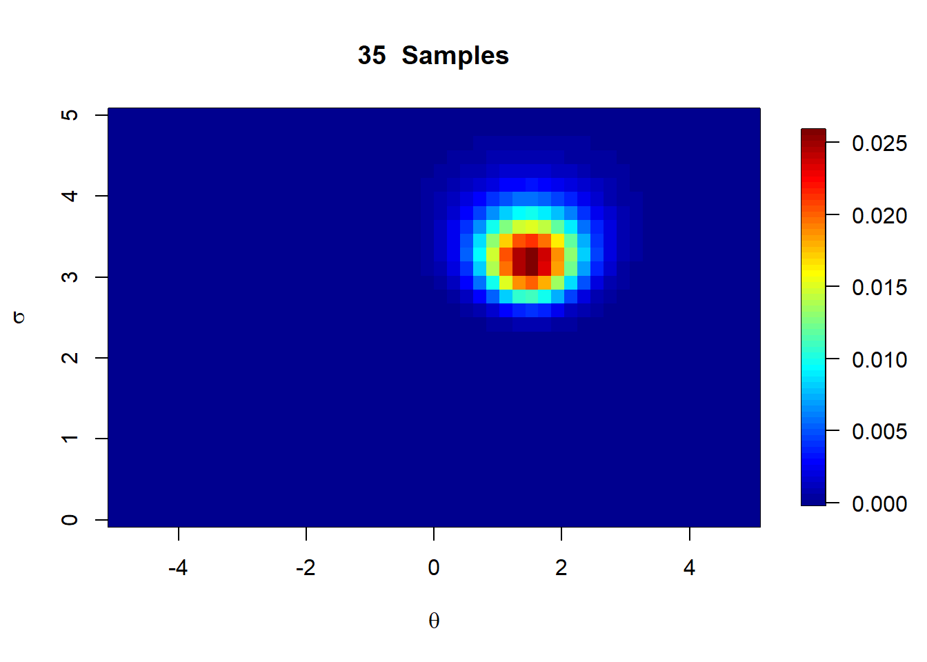
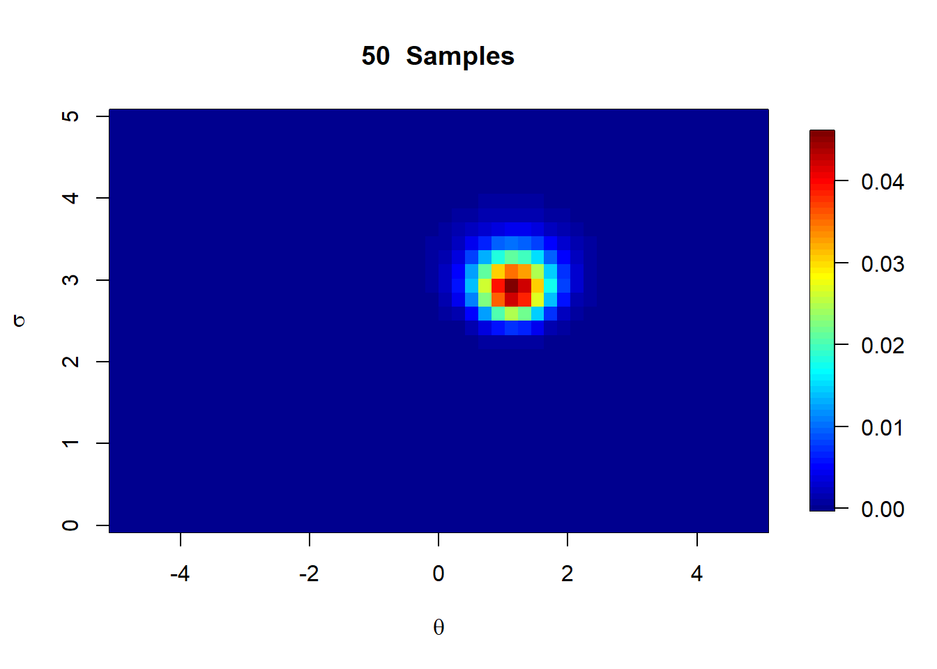
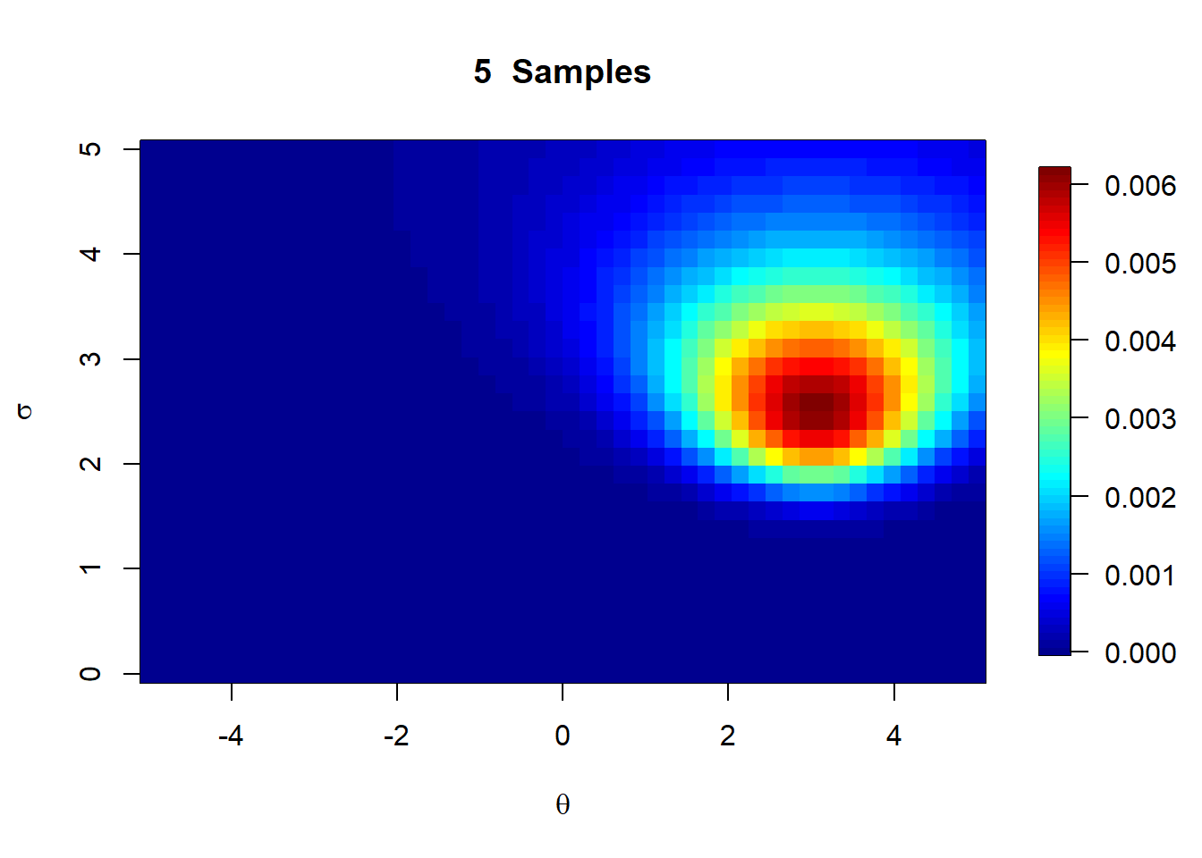
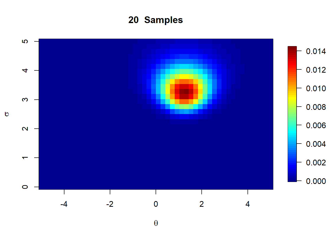
for(n1 in seq(5,n,by =  15)){
  estimates <- post_approx(y[1:n1],n1,mu_range,s_range)
  #Normalize Posteriors as densities are quite small
  estimates <- estimates/sum(estimates)


  image.plot(mu_range,s_range,estimates,
           xlab=expression(theta),
           ylab=expression(sigma),
           main = paste(n1," Samples"))
  #contour(mu_range,s_range,estimates,add=T)
}

We can see that our posterior does a reasonable job of picking up the true parameters from the data when using an improper prior once enough samples are included.

10.1.3.1 Example #3 Marginal Posterior Distribution - Mean

We can now marginalize the posterior to be able to get the marginal posteriors for \(\theta\) and \(\sigma^2\). In practice this is quite simple (usually). All that is required is to integrate the full posterior over the parameter space of the nuisance parameter (in this case, \(\sigma^2\).

\[ p(\theta|y) = \int_0^\infty p(\theta,\sigma^2|y)d\sigma^2 \]

\[ = \int_0^\infty p(y|\theta,\sigma^2)p(\theta,\sigma^2)d\sigma^2 \]

In this setting, we define the joint prior as follows:

\[ p(\theta,\sigma^2) = p(\theta |\sigma^2)p(\sigma^2) \]

Where

\[ p(\theta |\sigma^2) \sim Normal(\mu,\sigma^2/\lambda) = \frac{1}{\sqrt{2\pi \frac{\sigma^2}{\lambda}}} \exp\left(-\frac{(\theta - \mu)^2}{2 \frac{\sigma^2}{\lambda}}\right) \]

\[ p(\sigma^2) \sim InvGamma(\alpha,\beta) = \frac{\beta^\alpha}{\Gamma(\alpha)} (\sigma^2)^{-(\alpha + 1)} exp\left({-\frac{\beta}{\sigma^2}}\right) \]

\[ p(\theta,\sigma^2) \propto \]

The full posterior is therefore

\[ p(\theta,\sigma^2 | y) \propto \]

\[ p(\theta|y) = \int_0^\infty p(\theta,\sigma^2|y)d\sigma^2 \propto \int_0^\infty \]

10.2 Hierarchical Models