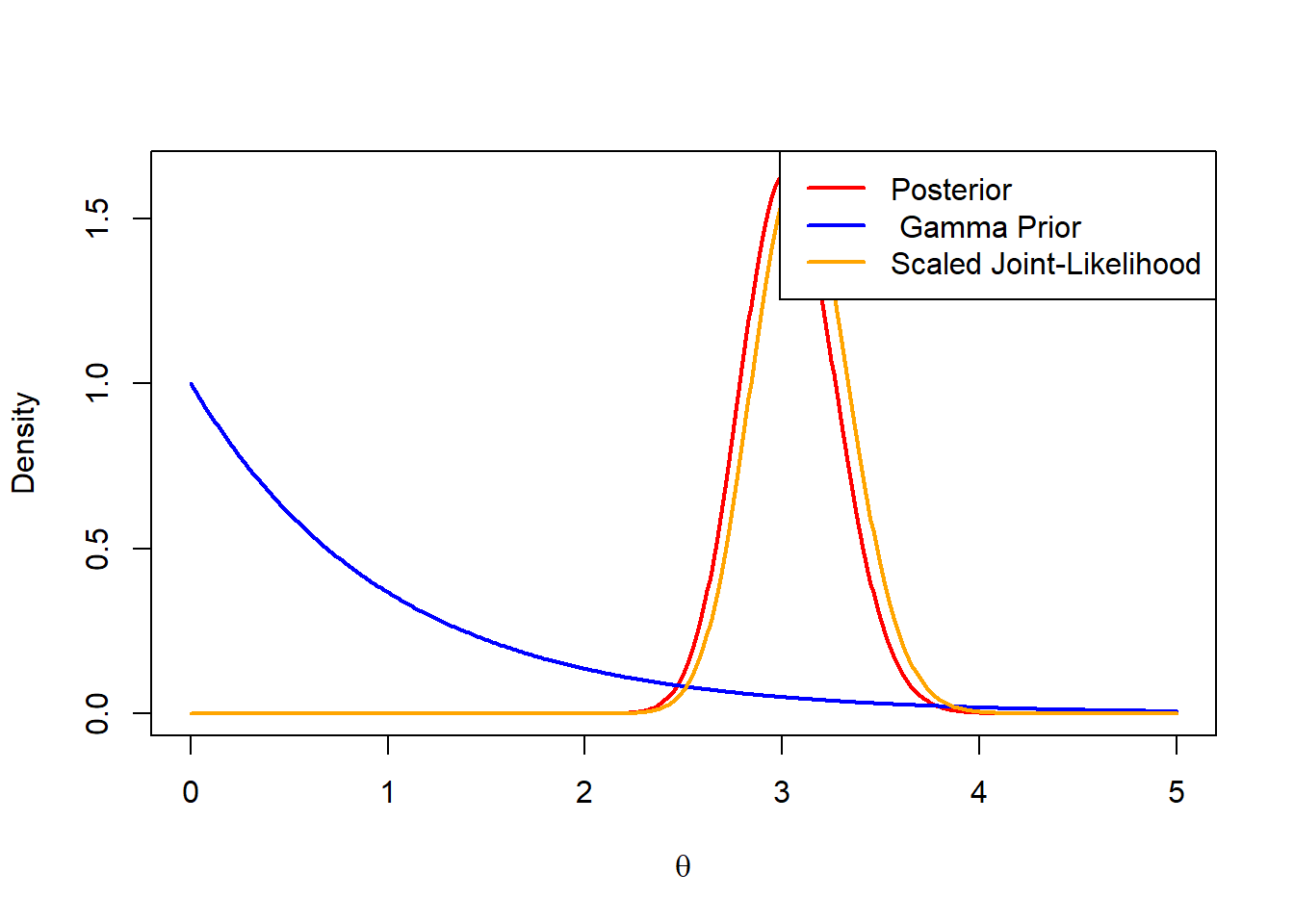
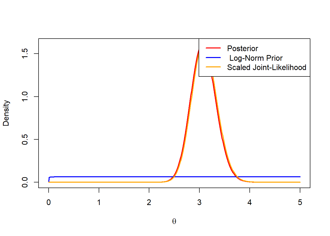
Explore the posterior density \(\pi_n(\theta)\) using two priors
\(Gamma(\alpha_0,\beta_0)\)
prior determined by the assumption that \(\phi = log\theta \sim Normal(\eta_0,\tau_0^2)\) a priori. In other words, that the prior is a log-normal distribution
We have the following observations
y
0
1
2
3
4
5
6
Count
2
6
7
16
11
6
2
Assuming that the likelihood is independent given\(\theta\) (de Finetti), multiplying the joint likelihood by the Gamma prior gives us a Gamma posterior with observation-dependent parameters (due to gamma-poisson conjugacy - see Conjugate Distributions).
We can now plot the posterior over all possible \(\theta \in \Theta\).
a <-1b <-1y <-c(rep(0,2),rep(1,6),rep(2,7),rep(3,16),rep(4,11),rep(5,6),rep(6,2))s_n <-sum(y)n <-length(y)theta <-seq(0,5,by =0.01)ll <-sapply(theta,function(thet){prod(dpois(y,thet))})#scalling likelihood to be visible in plotM <-max(dgamma(theta,a+s_n,b+n))/max(ll)plot(theta,dgamma(theta,a+s_n,b+n),type ='l',col ='red',lwd =2,xlab =expression(theta),ylab ='Density')lines(theta,dgamma(theta,a,b),col ='blue',lwd =2)lines(theta,ll*M,col ='orange',lwd =2)legend('topright',legend =c('Posterior',' Gamma Prior','Scaled Joint-Likelihood'),col =c('red','blue','orange'),lwd =2)
eta <-0tau <-10#Can treat the joint-likelihood as a gamma dist with a = sn and b = n to avoid need for individual observationslnorm_pois <-function(eta,tau,theta,sn,n){ calc <-dgamma(theta,sn,n)*dnorm(log(theta),eta,tau)return(calc)}norm_const <-integrate(lnorm_pois,eta = eta,tau =tau,sn = s_n,n = n,lower =0, upper =10)M <-max(lnorm_pois(eta,tau,theta,s_n,n)/norm_const$value)/max(ll)S <-max(lnorm_pois(eta,tau,theta,s_n,n))/max(dnorm(log(theta),eta,tau))plot(theta,lnorm_pois(eta,tau,theta,s_n,n)/norm_const$value,type ='l',col ='red',lwd =2,xlab =expression(theta),ylab ='Density')lines(theta,dnorm(log(theta),eta,tau)*S,col ='blue',lwd =2)lines(theta,ll*M,col ='orange',lwd =2)legend('topright',legend =c('Posterior',' Log-Norm Prior','Scaled Joint-Likelihood'),col =c('red','blue','orange'),lwd =2)