This section contains very basic examples of R code for Single cell analyses using 10X data.
Examples in this section were made using the OSCA e-book and data from the 10X Genomics Dataset Page. Pancreas datasets came from the Grun et al. and Muraro et al. papers.
6.2 1. Loading 10X Data into R
We can load 10X Data into R to generate a ‘SingleCellExperiment’ object. We can either
load the cellranger outputs directly
set.seed(1234)library(DropletUtils)
Loading required package: SingleCellExperiment
Loading required package: SummarizedExperiment
Loading required package: MatrixGenerics
Loading required package: matrixStats
Warning: package 'matrixStats' was built under R version 4.2.3
The following objects are masked from 'package:base':

    expand.grid, I, unname
Loading required package: IRanges
Attaching package: 'IRanges'
The following object is masked from 'package:grDevices':

    windows
Loading required package: GenomeInfoDb
Loading required package: Biobase
Welcome to Bioconductor

    Vignettes contain introductory material; view with
    'browseVignettes()'. To cite Bioconductor, see
    'citation("Biobase")', and for packages 'citation("pkgname")'.
Attaching package: 'Biobase'
The following object is masked from 'package:MatrixGenerics':

    rowMedians
The following objects are masked from 'package:matrixStats':

    anyMissing, rowMedians
#Load raw cellranger counts#file.name <- "../Data/raw_gene_bc_matrices/GRCh38/"#You can also load the filtered counts (removes empty droplets)file.name <-"../Data/filtered_gene_bc_matrices/GRCh38/"sce <-read10xCounts(file.name)
'as(<dgTMatrix>, "dgCMatrix")' is deprecated.
Use 'as(., "CsparseMatrix")' instead.
See help("Deprecated") and help("Matrix-deprecated").
#read10xCounts takes a directory path and looks for the three key 10X outputs#barcodes.tsv, genes.tsv, matrix.mtxsce
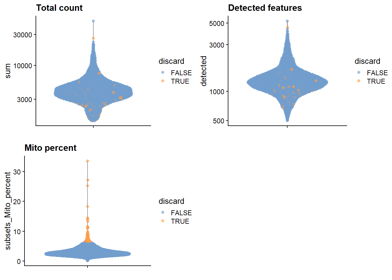
#Practice Add metadata column that says which cells have at least 1500 detected genes#Practice Add metadata column that says which cells have at least 10 detected mitochondrial genes
6.3.4 Normalization
library(scran)set.seed(1234)clusters <-quickCluster(sce) #Simple way to generate clusterssce <-computeSumFactors(sce, cluster=clusters)sce <-logNormCounts(sce)dec <-modelGeneVar(sce)top_hvgs <-getTopHVGs(dec,n =2000)
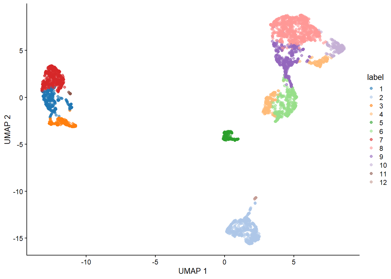
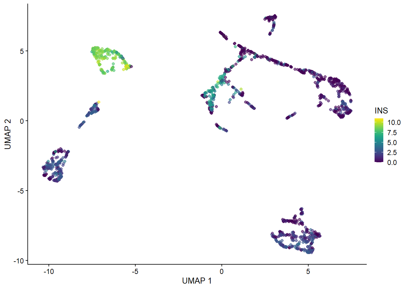
6.4 3. Dimension Reduction & Clustering
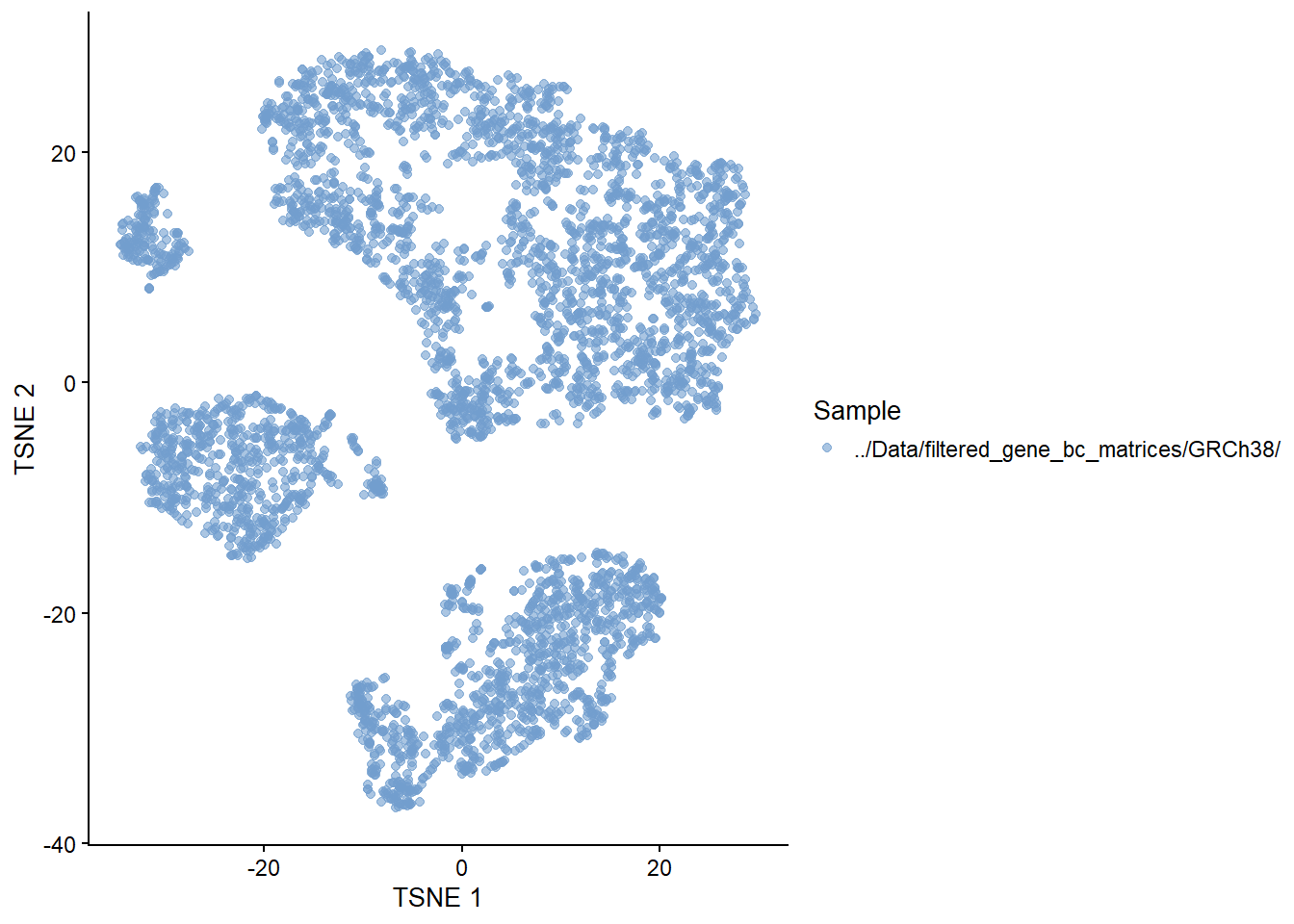
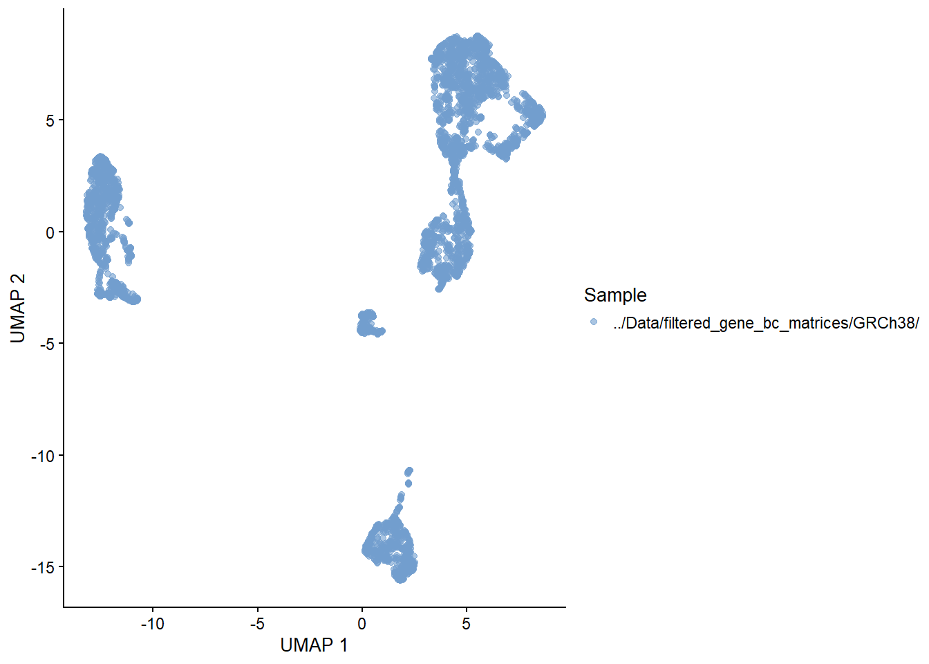
Dimension reduction is extremely useful for visualizing single cell data. Although PCA is still viable, it does not perform as well as non-linear methods such as t-SNE and UMAP. Do note that although UMAP is currently the tool of choice, there is currently a big debate on the benefits of using such methods in analysis (I suggest looking up Lior Pachter’s work to learn more about this).
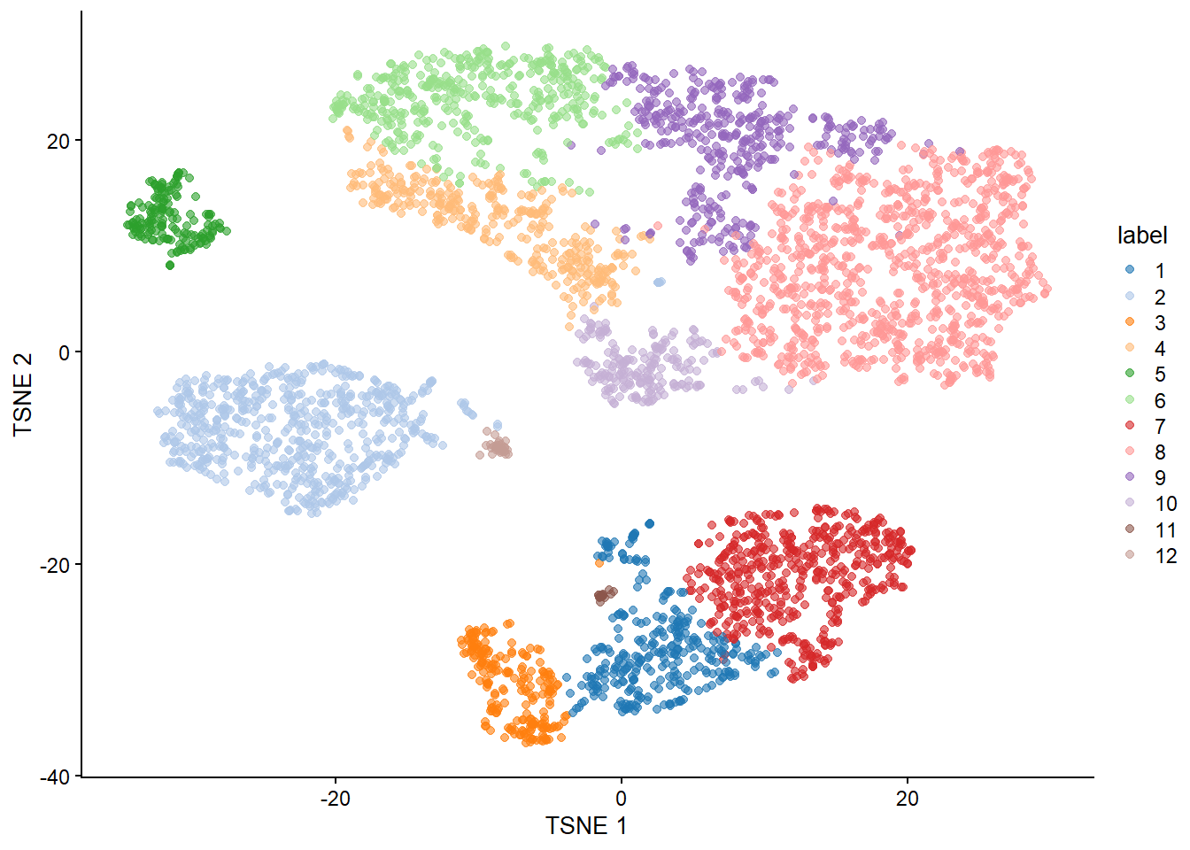
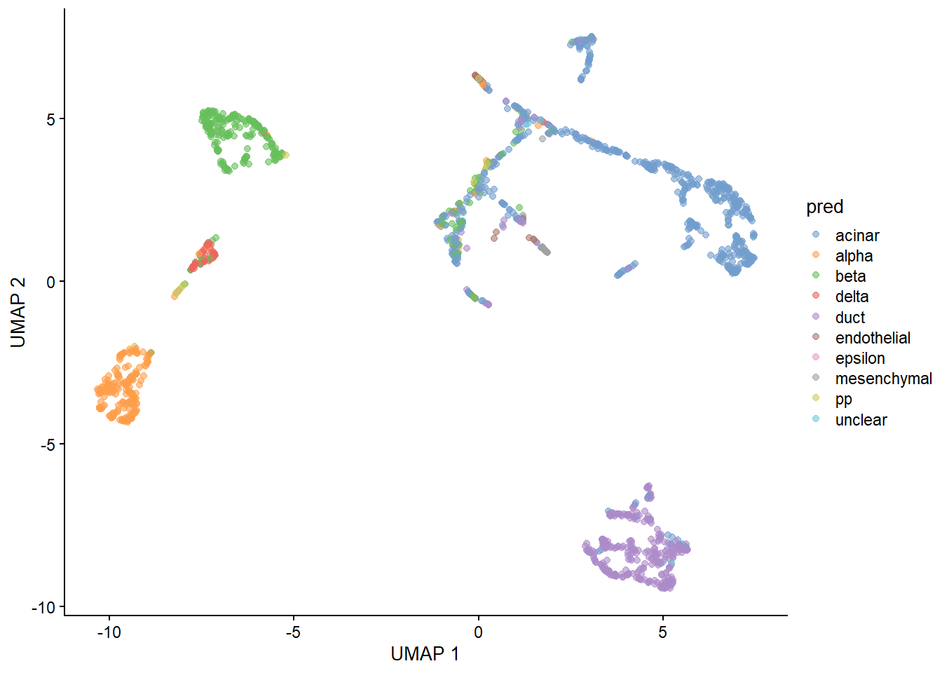
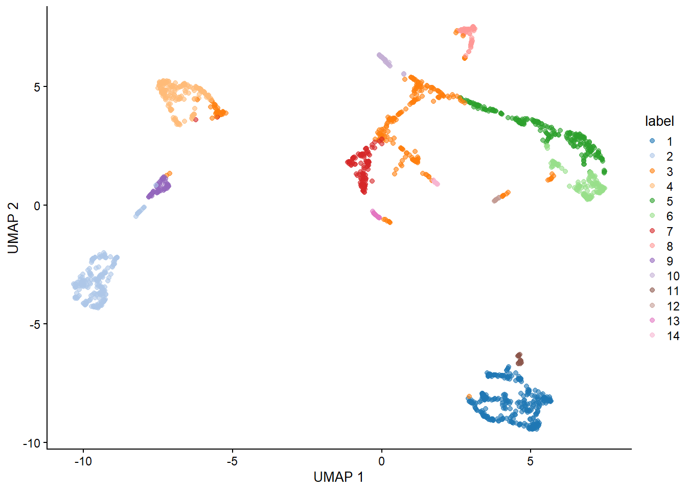
With our generated UMAP coordinates and clusters, we can undertake the task of cell annotation. It is possible to do this manually and automatically. In practice, I suggest to combine both approaches to ensure your annotations are as accurate as possible. In this section we will use pancreas samples.
6.5.1 Automated Annotation
A key advantage of automated annotation is that it usually (depending on the method) provides an annotation for individual cells. This is quite useful for scoring individual cells and identifying sub cell types.
An issue with labeling individual cells is that their annotation is more susceptible to noise. To this end, manual annotations which are usually done at the level of clusters may be more reliable.
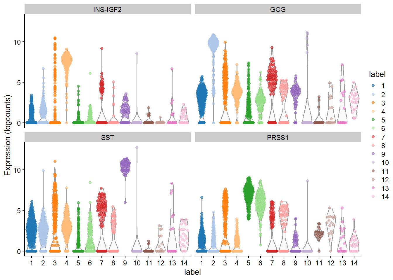
6.5.3 Considerations for DGE during cluster annotation
Previously, many researchers would simply run a DGE analysis on different clusters to determine cell types. However, this has been proven to be a case of ‘double-dipping’ data which is a serious concern for reproducibility. Although this approach can work fine for very distinct cell types, it is not recommended for the analysis of more similar cell types of cell subtypes.